Propagation Modeling
Characterize the radio channel directly from real-world city geometry.
How the workflow runs
Place an antenna in the city, sweep a grid of field points, and extract the real part of the Poynting vector as a proxy for time-averaged received power. Regress against distance to find the pathloss exponent and pathloss at 1 m, and fit a normal distribution to recover the log-normal shadow variance.
Place two antennas in the city geometry and compute the frequency-domain channel between them. An inverse Fourier transform into the delay domain yields the impulse response and the power delay profile.
Build a receive antenna array and one or more transmitters. From the channel vector or matrix, a 1-D DFT (uniform linear array) or 2-D DFT (uniform planar array) resolves multipath magnitude against angle of arrival.
Large-Scale Modeling
Recover the pathloss exponent and log-normal shadowing from a grid of field points above the terrain.
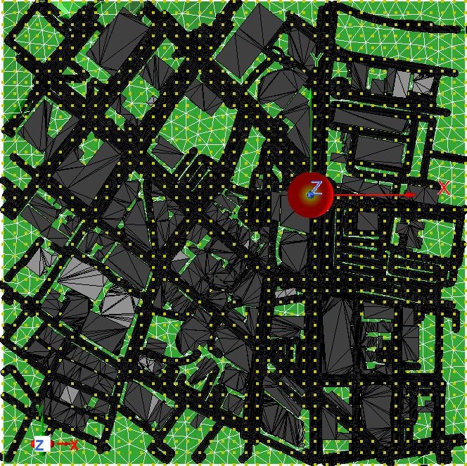
Place an antenna at the desired location in the city geometry and choose the directivity pattern — here an omnidirectional dipole at 5 GHz. A grid of points is created above the terrain where the Poynting vector is evaluated.
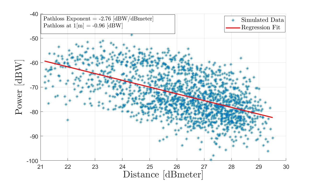
Extract the real part of the Poynting vector at every grid point and regress to obtain the pathloss exponent and pathloss at 1 m. In this example the exponent is −2.76; free-space power decay has an exponent of −2.
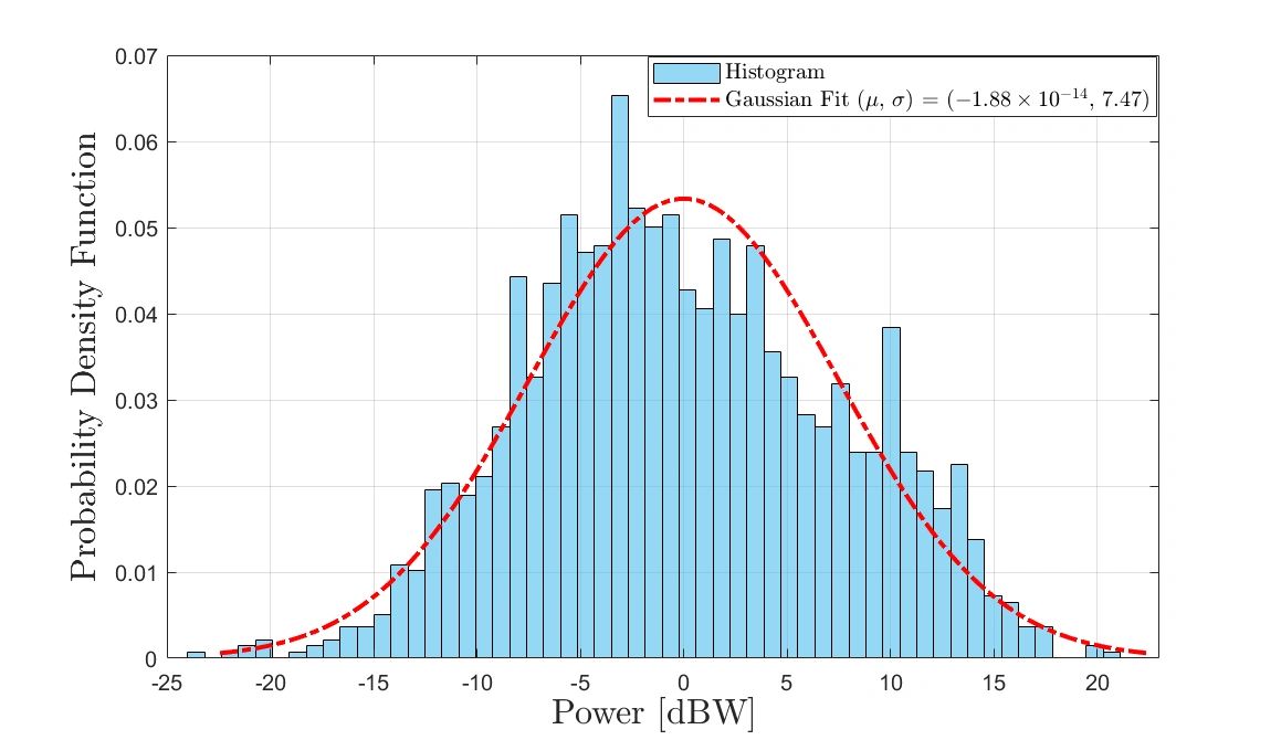
Estimate the standard deviation of the zero-mean Poynting-vector data and fit it to a normal distribution. Here the shadowing standard deviation is 7.47 dB.
Small-Scale Modeling
Extract the impulse response and power delay profile between a transmitter and receiver placed in the city.
Create a setup with a single-antenna transmitter and a single-antenna receiver — here two Hertzian dipoles — at chosen locations in the city. The carrier is 5 GHz with 100 MHz of channel bandwidth.
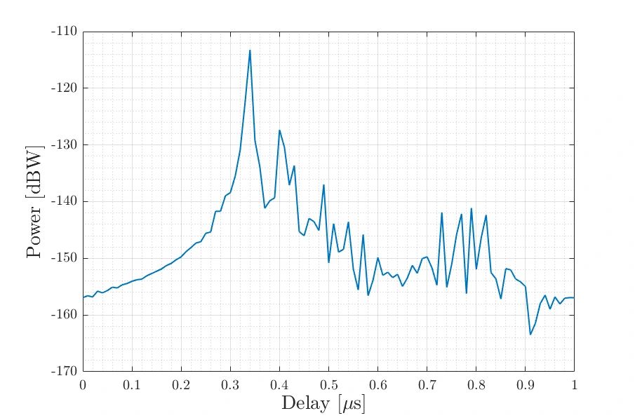
Calculate the PDP in dBW against delay in microseconds. The channel shows a frequency-flat response with the main tap at ≈0.3 µs — at the speed of light, a transmitter–receiver separation of about 90 m.
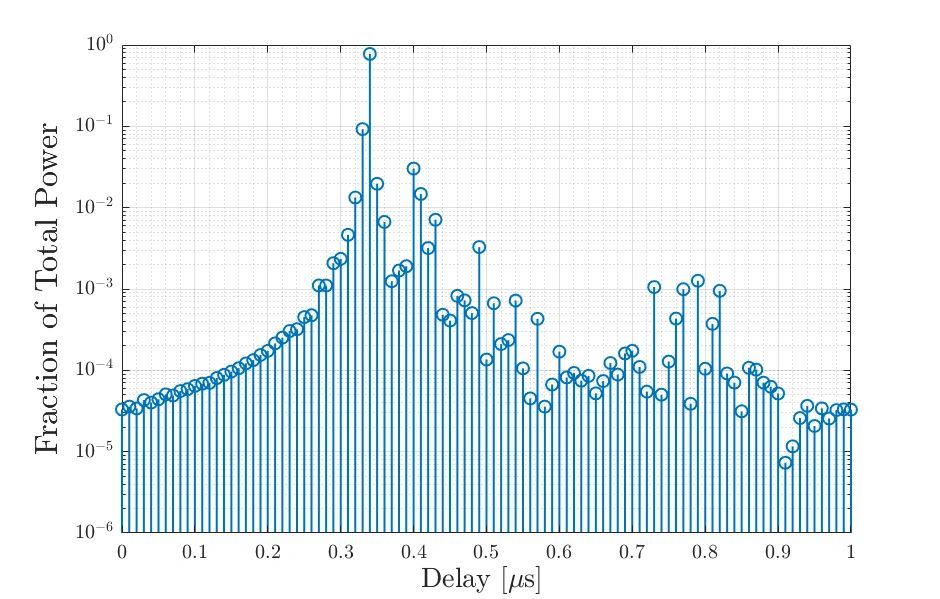
Normalize the PDP so total channel power is one and each tap is a fraction of the total. The main tap sits at least 10 dB above the second-largest tap.
Localization
Resolve the angle of arrival of a transmitter from a receive antenna array.
Create a receiver with a 16-element uniform linear Hertzian-dipole array and a transmitter with a single Hertzian dipole.
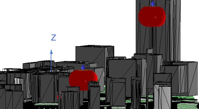
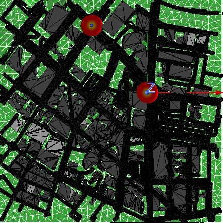
Place the receiver at an elevation relative to the transmitter within the city geometry.
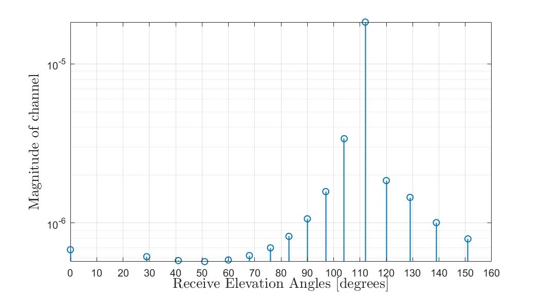
Obtain the channel vector and compute a 1-D DFT. Plotting multipath magnitude against angle of arrival picks out the strongest path — here the transmitter resolves at 112° relative to the receiver, consistent with the setup.
Run this workflow on your geometry
WirelessAI agents set up and run this study on top of your Ansys Electronics Desktop environment — no Python required.